Teaching a neural network to draw
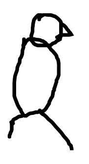
Can you draw a penguin in less than 20 seconds?
If so, check out Google Quick Draw!, a game that asks you to do exactly that. If not, you are in luck, because this article is about teaching a neural network to do it for you.
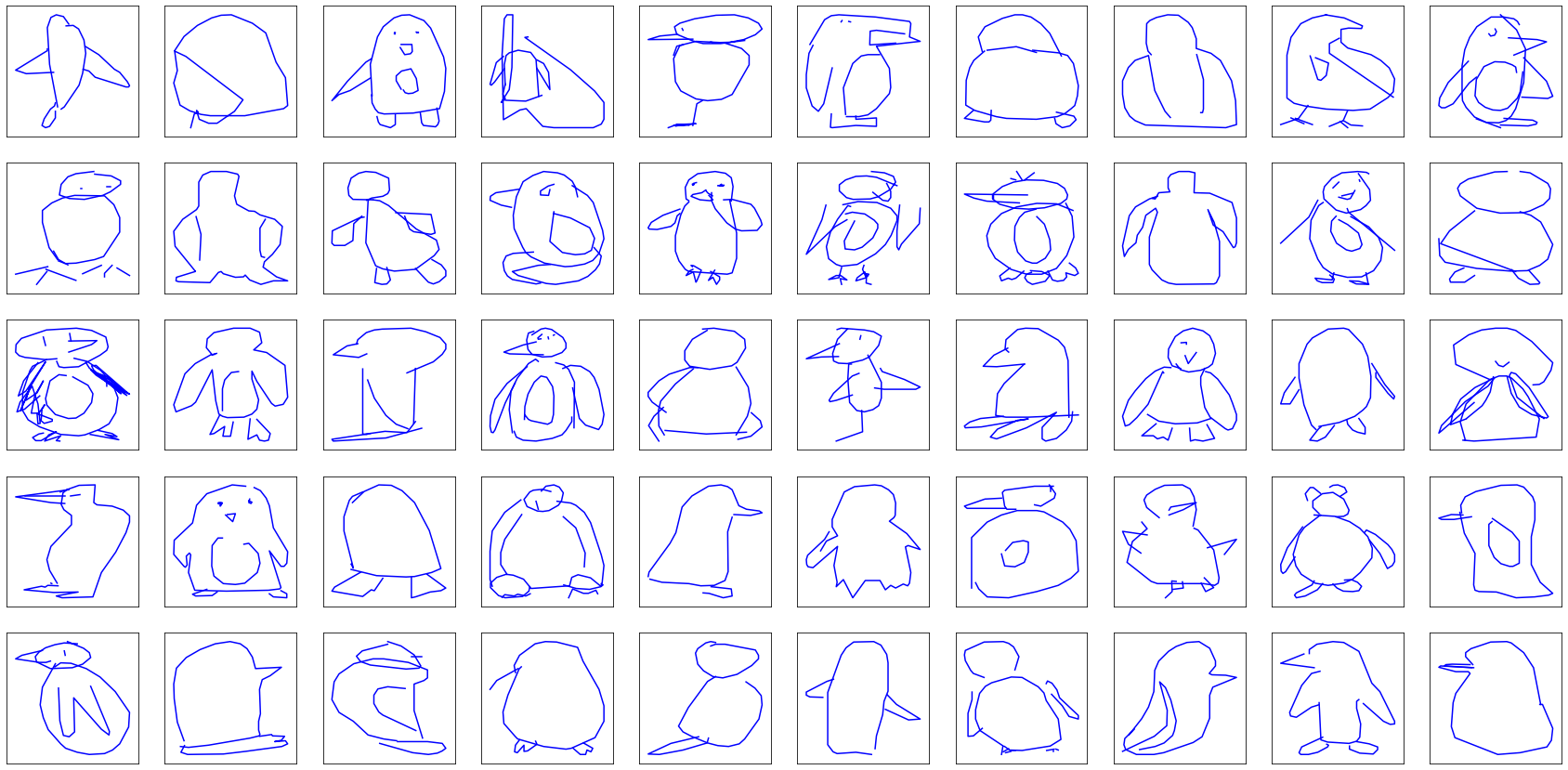
(click the image for more samples)
Quite amazingly, a lot of the generated sketches outcompete the ones the machine learned to draw from.
The article explains what the model generating the drawings looks like. The code (Pytorch) is available on Github.
Note: Throughout the article, everytime a series of 5 drawings is presented, the image links to the larger series they were chosen from. Feel free to click it to see how biased (or not) the selection is.
Structure of the article
Let’s start at the end.
Concretely, the model is a recurrent neural network that jointly decides the position of each point, when to lift the pencil, and when to stop drawing. In order to better account for the uncertainty of hand-drawn trajectories, the network does not output the points directly. Instead, it outputs the parameters of some probability distributions from which the position and nature of the points can be sampled. The model is trained using gradient descent over a loss function that maximizes the likelihood of said distributions given the points in the training set.
I’m aware that last paragraph might not appear as crystal clear to most readers. If it is for you, you can refer directly to the Google Brain paper that describes the model, referred to as “unconditional generation of drawings”.
For the rest of us, this article gives a shot at explaining as simply as possible the various parts of the model: the neural net part, the probabilistic layer stacked on top of it, and how they fit together.
Expect to see a lot of crappy drawings along the way, in search for the final model.
Data
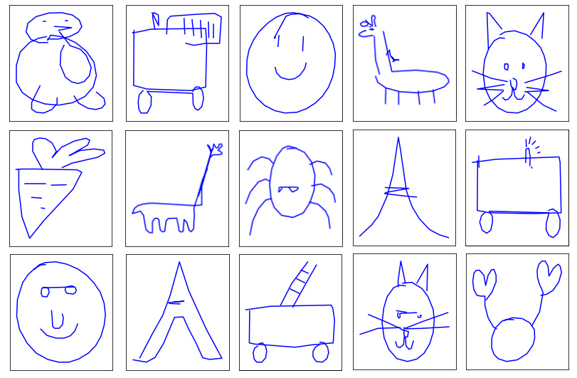
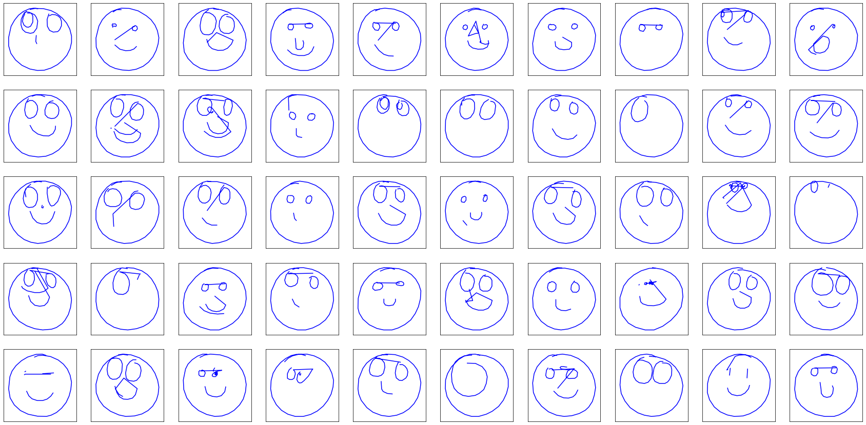
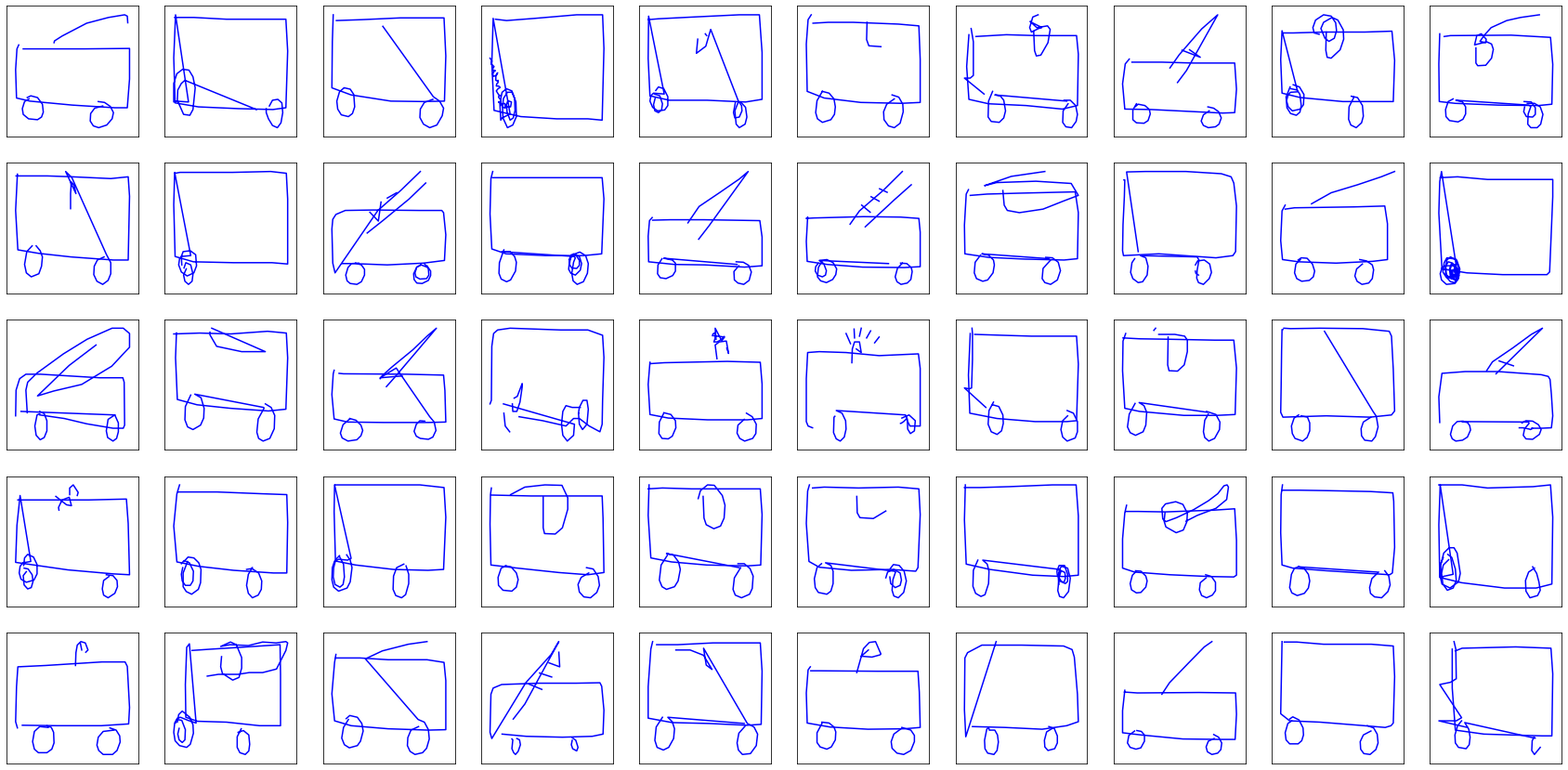
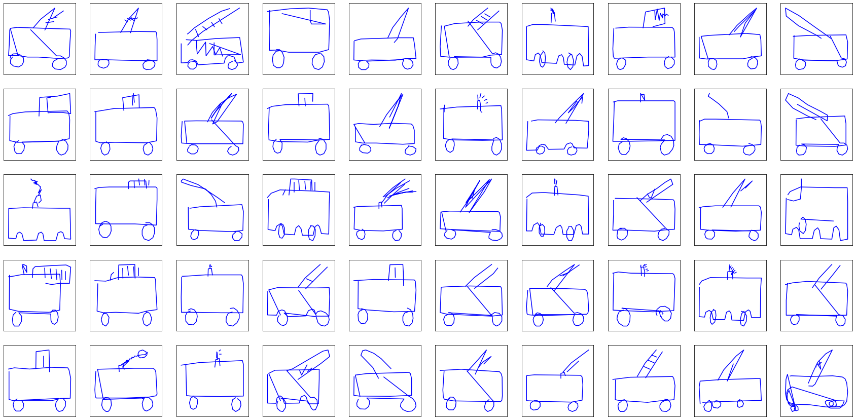
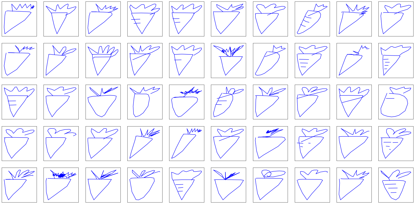
The dataset consists in 50 million drawings available through Github across 345 categories. Let’s pick 3 of them (Eiffel tower, face and fire truck) and attempt to model them. Here is an excerpt of the dataset:
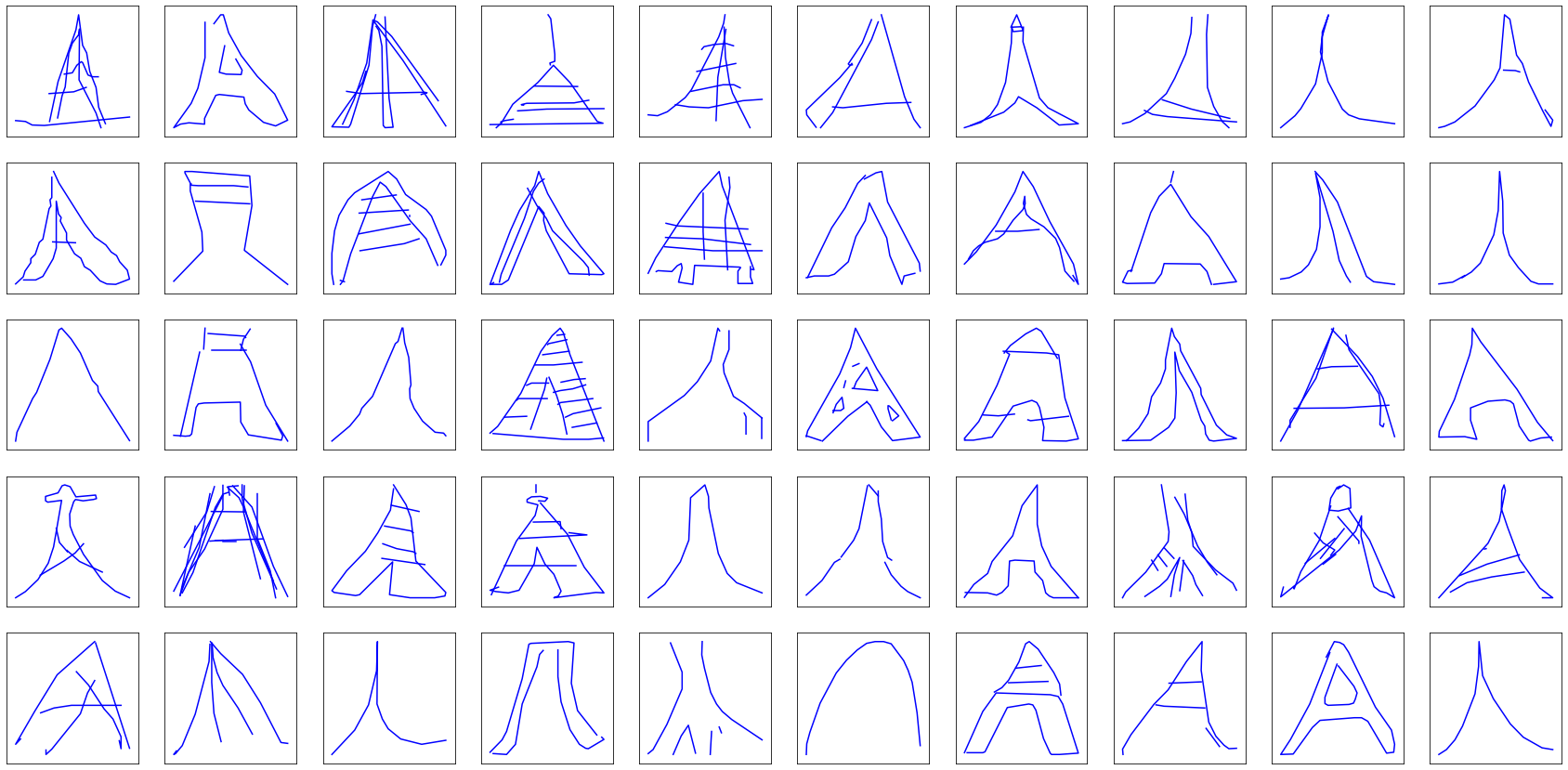
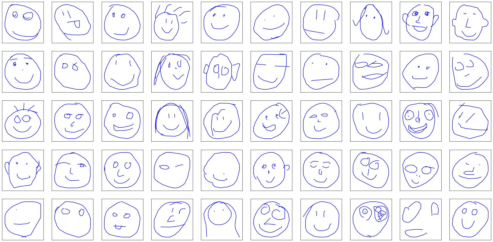
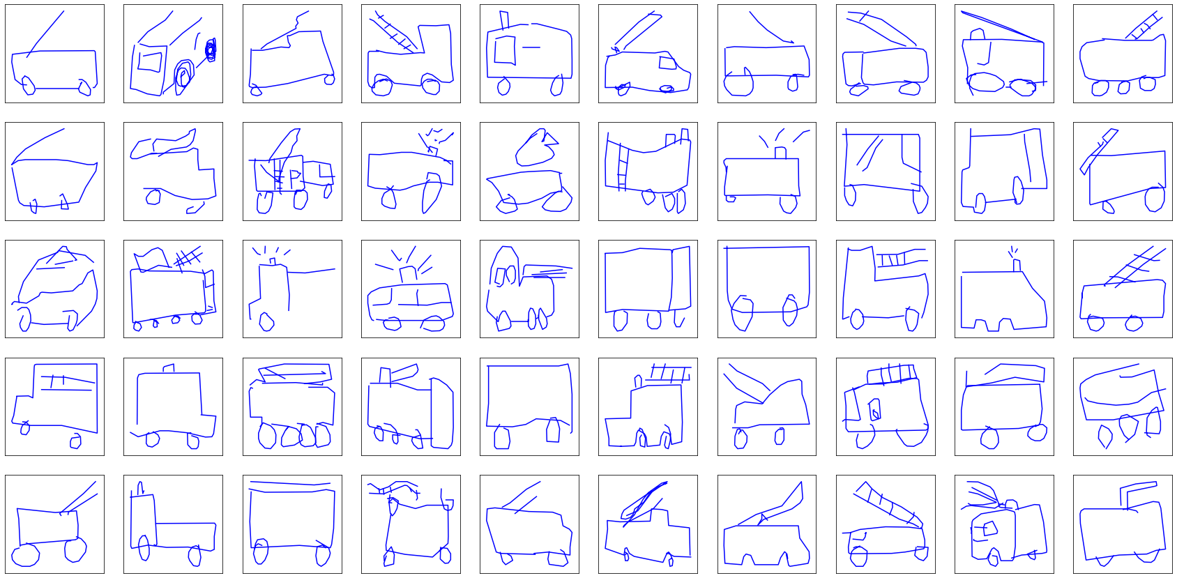
All three categories provide a different set of challenges. Eiffel towers contain mostly-continuous strokes with some sharp changes in directions. Faces are smoother, though it is probably more difficult to position the various strokes with respect to each other. Fire trucks are definitely the most difficult to draw, combining the previous difficulties of Eiffel towers and faces with even more strokes.
Drawings as sequences of points
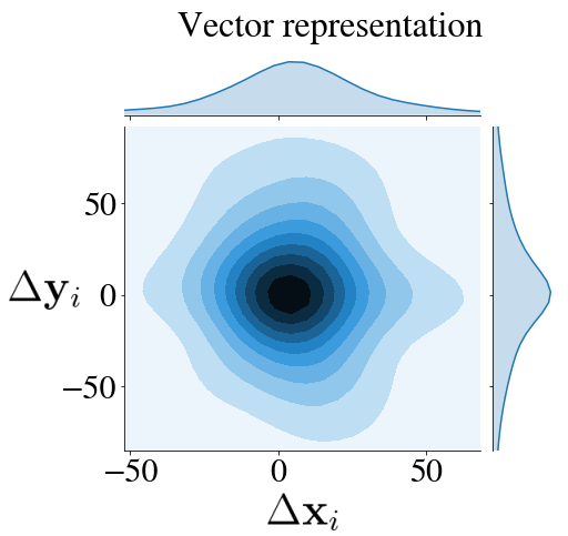
Drawings are presented in the dataset in their most obvious shape: sequences of points $\begin{bmatrix} \mathbf{x}_{i},~\mathbf{y}_{i} \end{bmatrix}$. But it is not the only way to represent them. What about sequences of vectors $\begin{bmatrix} \Delta \mathbf{x}_{i},~\Delta \mathbf{y}_{i} \end{bmatrix}$ from each points to the next, or — let’s get crazy — sequences of polar-coordinates vectors $\begin{bmatrix} \mathbf{r}_{i},~\mathbf{\theta}_{i} \end{bmatrix}$ from one vector to the next?
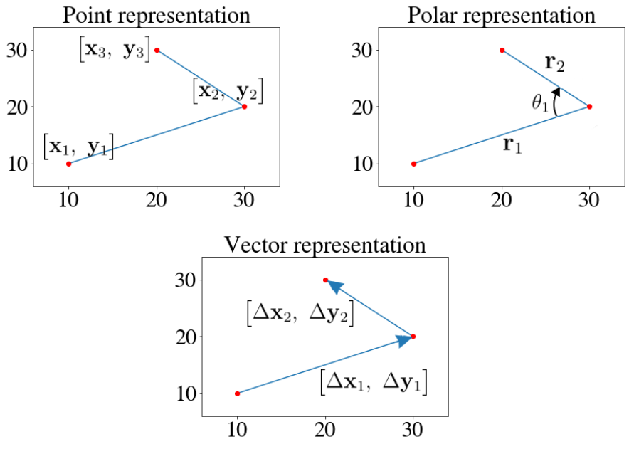
It turns out the vector representation is the most interesting for at least three reasons:
- It is trivial and inexpensive to compute: $\begin{bmatrix} \Delta \mathbf{x}_{i},~\Delta \mathbf{y}_{i} \end{bmatrix} = \begin{bmatrix} \mathbf{x}_{i+1} - \mathbf{x}_{i},~\mathbf{y}_{i+1} - \mathbf{y}_{i} \end{bmatrix}$ , as opposed to the polar representation I will spare you the trigonometry of.
- It allows us to define a compelling object: a no-displacement vector $\overrightarrow 0 = \begin{bmatrix} 0,~0 \end{bmatrix}$. It has no equivalent in the original point representation, where $\begin{bmatrix} 0,~0 \end{bmatrix}$ is just a regular point. It does in the polar representation, but not without a few caveats. For instance, what should the angle between $\overrightarrow 0$ and another vector be?
-
It is the only representation in which the points follow a distribution, which, although too spread out to be gaussian, is at least symmetrical.
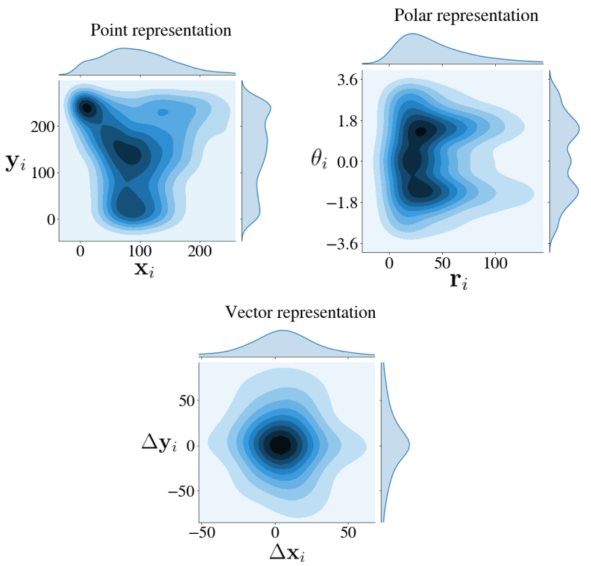
In order for the neural net to learn more effectively, we are going to standarize each point by the mean $\begin{bmatrix} \mathbf{\mu}_1,~\mathbf{\mu}_2 \end{bmatrix}$ and standard deviation $\begin{bmatrix} \mathbf{\sigma}_1,~\mathbf{\sigma}_2 \end{bmatrix}$ of all point in the whole dataset:
$$ \begin{bmatrix} \Delta \mathbf{x}_{i},~\Delta \mathbf{y}_{i} \end{bmatrix}= \begin{bmatrix} \frac{\Delta \mathbf{x}_{i} - \mu_1}{\sigma_1}, ~\frac{\Delta \mathbf{y}_{i} - \mu_2}{\sigma_2} \end{bmatrix} $$
It makes much sense when the mean and variance correspond to the actual center and spread of a symmetrical distribution.
So we pick the $\begin{bmatrix} \Delta \mathbf{x}_{i},~\Delta \mathbf{y}_{i} \end{bmatrix}$ representation and carry on.
In order not to clutter all subsequent equations with $\Delta$’s, though, let’s discard them. From now on, and until the end of the article, $\begin{bmatrix} \mathbf{x}_i,~\mathbf{y}_i \end{bmatrix} = \begin{bmatrix} \Delta \mathbf{x}_i,~\Delta \mathbf{y}_i \end{bmatrix}$. We will refer to the these vectors as “point” wherever convenient.
Model
As per the previous paragraph, each drawing $\mathcal{X}$ is a sequence of 2-dimensional displacement vectors $\mathcal{X}_i = \begin{bmatrix} \mathbf{x}_{i},~\mathbf{y}_{i} \end{bmatrix}$ with its own length $N-1$, since each vector compacts every successive points of the original drawing into one.
Our goal is to create a model that can generate such drawings. Concretely, it means we are looking for a function $f$ that takes a vector $\mathcal{X}_i = \begin{bmatrix} \mathbf{x}_i,~\mathbf{y}_i \end{bmatrix}$ as input, and returns a prediction $\mathcal{\hat Y}_i = \begin{bmatrix} \mathbf{\hat x}_{i+1},~\mathbf{\hat y}_{i+1} \end{bmatrix}$ for what the next vector should be. The hat $\hat~$ denotes the output of the model, as opposed to actual vectors from the dataset.
With such a model at hand, generating a drawing can be approached as an iterative process:
- pick up an initial vector $\mathcal{X}_{i=1}$ as the current one
- predict the next vector $\mathcal{\hat Y}_i = f(\mathcal{X}_i)$
- use the prediction as the current vector
- go back to step 2

In order to skip picking up the first point, let’s make all drawings start with the same additional vector $\mathcal{X}_1 = \overrightarrow 0$, ending up with nicely aligned sequences $\mathcal{X}$ and $\hat{\mathcal{Y}}$ of length $N$.
Feedforward neural network
$f$ is not an arbitrary function. Quite naively, let us consider it is a feedforward neural network ($f = nn_{_W}$) with a hidden layer of size $H = 128$ and hyperbolic tangent ($tanh$) activation function. If you’re fuzzy on what it means, don’t run away. What is inside $nn_{_W}$ is much less relevant than how we interact with it from the outside. Put another way: feel free to consider it a black box.
$$ \begin{aligned} &\text{1-hidden-layer neural network:} \\ &~~~~~~nn_{_W}(\mathcal{X}_i) = \mathbf{W_O} \times \mathbf{h} + \mathbf{b_O} \\[5pt] &\text{With hidden state:} \\ &~~~~~~~~\mathbf{h} = \tanh( \mathbf{W_I} \times \mathcal{X}_i + \mathbf{b_I}) \\[5pt] &\text{And parameters:} \\ &~~~~~~\mathbf{W_I}\text{~~~~input weights~~~~~(matrix or size }2 \times H\text{)} \\ &~~~~~~\mathbf{W_O}\text{~~~output weights~~~(matrix or size }H \times H\text{)} \\[8pt] &~~~~~~\mathbf{b_I}\text{~~~~~input bias~~~~(column vector of size }H\text{)} \\ &~~~~~~\mathbf{b_O}\text{~~~~output bias~~(column vector of size }H\text{)} \\ \end{aligned} $$
All there is to understand is that given a bunch of weight $W$, the neural network is a function $nn_{_W}$ that associate to each input $X_i$ a given output $\mathcal{\hat Y}_i$. On the way, it computes an internal vector $\mathbf{h}$ whose size $H$ conditions the complexity of $nn_{_W}$. Since matrix multiplications and sums are linear operations, throwing a $tanh$ into the mix ensures the resulting function is more than just a linear one.
Training
To achieve any kind of meaningful generation with $nn_{_W}$, we first need to train it. Concretely, it means that we are looking for a set of weights $W$ that make each prediction $\mathcal{\hat Y}_i$ as close as possible from the “true next vector” $\mathcal{Y}_i = \mathcal{X}_{i+1}$ as available in the dataset. Those vectors are the labels: $\mathcal{Y} = \mathcal{Y}_1~…~\mathcal{Y}_N$.
That leaves us with a supervised auto-regression problem: supervised because there are labels, regression because those labels are real-valued, and auto because they are essentially the same as the data: $\mathcal{Y}_i = \mathcal{X}_{i+1}$.
In order to quantify how close the predictions are from the labels, we need to define a loss function $\mathscr{L}(\mathcal{\hat{Y}},\mathcal{Y})$, such as the average sum of squated distances between each data point and label known as the mean-squared error (MSE):
$$ MSE(\hat{\mathcal{Y}},\mathcal{Y}) = \frac{1}{N - 1} \sum_{i=1}^{N-1} \left[ (\mathbf{\hat{x}}_{i+1} - \mathbf{x}_{i+1}) ^ 2 + (\mathbf{\hat{y}}_{i+1} - \mathbf{y}_{i+1}) ^ 2 \right] $$
The smaller the value of $MSE(\mathcal{\hat Y},\mathcal{Y})$, the closest the generated drawing $\mathcal{\hat Y}$ is from the original drawing $\mathcal{Y}$. If it is $0$, then $\mathcal{\hat Y} = \mathcal{Y}$. Overfitting is not an issue here, since we do not care about generalization, but about accurate generation.
To summarize, given a dataset of $M$ drawings $\mathcal{X}$ and their corresponding labels $\mathcal{Y}$, training $nn_{_W}$ means finding a set of weights $W_{optimal}$ such as:
$$ W_{optimal} = \underset{W}{\argmin}~ \frac{1}{M} \sum_{(\mathcal{X},~\mathcal{Y})} MSE(nn_{_W}(\mathcal{X}),~\mathcal{Y}) $$
In practice, $W_{optimal}$ is computed by gradient descent. Broadly speaking, gradient descent is about computing iteratively a sequence of weights $W_t$, that, for reasonable values of a parameter called the “learning rate” $\eta$ the strategy, converges to $W_{optimal}$. In practice, the learning rate conditions how aggressively $W_t$ is updated at each iteration.
$$ \begin{aligned} W_{t+1} = W_t - \eta \times \frac{\partial \mathscr{L}}{\partial W_t}(\mathcal{\hat Y}, \mathcal{Y}) \\[5pt] \text{where }\mathcal{\hat Y} = nn_{_{~W_t}}(\mathcal{X}) \end{aligned} $$
This equation (and its array of subtler variations) powers the whole edifice of deep learning edifice, effectively allowing neural networks to learn from data.
Although diving into the exact equations of gradient descent for $nn_W$ is out of the scope of this article, the key insight to gain from the equation is the following: the loss needs to be derivable with respect to the model parameters in order for the model to be trainable. Naturally, it is the case for MSE and feedforward neural networks.
Ideally, the drawings are fed in small batches to the neural networks (e.g. 64 drawings at a time), and an iteration of gradient descent is applied once at the end of each batch to adjust the weights. The process is repeated until all drawings of the dataset have been seen by the network, at which point it starts over (multiple epochs) until the loss value is satisfactory (low) enough.
For a great explanation of neural networks, how to train them without overfitting, how gradient descent works in details, and so much more, I couldn’t recommend enough the excellent (online) book Neural Networks and Deep Learning. It does not cover recurrent neural networks, however.
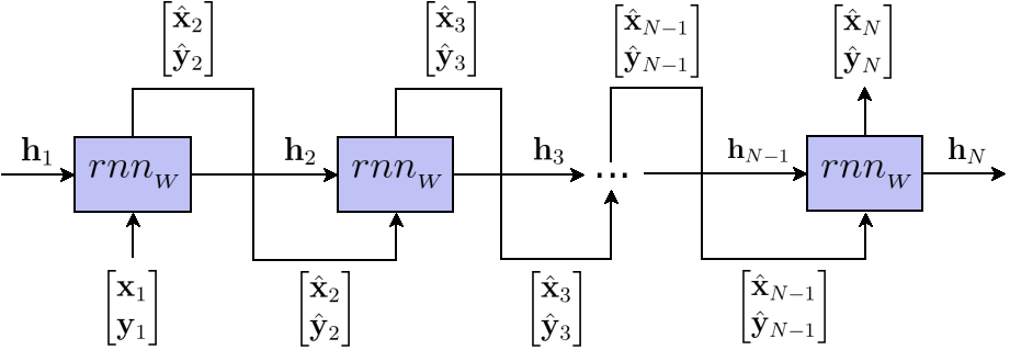
Recurrent neural networks
So far, so good. We have a model capable of learning from sequences of points and generating new ones. There is however, a minor caveat: it does not work. You can train it, pleasantly watch the loss go down, and the generation will fail at producing anything even remotely satisfying. Worse, it would probably reach better (smaller) losses by shuffling the drawings vectors. How on Earth is that possible?
I think you can see where it is going. The feedforward neural network merely takes the current vector as input, and it is a rather poor predictor for the next one. In order to take full advantage of the sequential structure of the data, we need a recurrent neural network.
The key idea that leads to RNNs is as follows: instead of feeding only the current vector $\mathcal{X}_i$ as input to the model, feed it all the previous vectors $\mathcal{X}_1~…~\mathcal{X}_{i-1}$ as well. Since a neural network accepts a fixed number of numbers as input, let us get clever and encode the previous vectors as a single vector $\mathbf{h}_i$ (called hidden state) of size $H$ (yes, the same $H$ wich is also the size of the hidden layer in our feedforward network).
The best is yet to come. How do we transform previous vectors $\mathcal{X}_1~…~\mathcal{X}_{i-1}$ to the hidden state? We don’t. The model does, and makes it available to the next step by outputting it.
$$ \begin{aligned} &\text{Recurrent neural network:} \\ &~~~~~~rnn_{_W}(\mathcal{X}_i {\color{Blue}{,~\mathbf{h}_i}}) = \mathbf{W_O} \times {\color{Blue}{\mathbf{h}_{i+1}}} + \mathbf{b_O} \\[5pt] &\text{With hidden state:} \\ &~~~~~~~~{\color{Blue}{\mathbf{h}_{i+1}}} = \tanh( \mathbf{W_I} \times \mathcal{X}_i + \mathbf{b_I}~ {\color{Blue}{+ \mathbf{W_H} \times \mathbf{h}_i + \mathbf{b_H}}}) \\[5pt] &\text{And parameters:} \\ &~~~~~~\mathbf{W_I}\text{~~~~input weights~~~~~(matrix or size }2 \times H\text{)} \\ &~~~~~~{\color{Blue}{\mathbf{W_H}\text{~~~hidden weights~~(matrix or size }2 \times H\text{)}}} \\ &~~~~~~\mathbf{W_O}\text{~~~output weights~~~(matrix or size }H \times H\text{)} \\[8pt] &~~~~~~{\color{Blue}{\mathbf{b_H}\text{~~~hidden bias~~(column vector of size }H\text{)}}} \\ &~~~~~~\mathbf{b_I}\text{~~~~~input bias~~~~(column vector of size }H\text{)} \\ &~~~~~~\mathbf{b_O}\text{~~~~output bias~~(column vector of size }H\text{)} \\ \end{aligned} $$
The blue parts highlight the differences with the feedforward neural network. Interestingly, it mainly comes down to updating and exposing as input the internal vector $\mathbf{h}_i$ that was already in the feedforward network as $\mathbf{h}$.
Again, the exact matrix multiplications and nonlinearities at play inside the network do not matter as much as how the model is used concretely.
The generation process is now as follows:
- pick up an initial point $\mathcal{X}_{i=1} = \overrightarrow 0$ as the current one, and an initial vector $\mathbf{h}_{i=1} = \overrightarrow 0$ as the current hidden state
- predict the next point and hidden state vector $\begin{bmatrix} \mathcal{\hat Y}_i,~\mathbf{h}_{i+1} \end{bmatrix} = rnn_{_W}(\mathcal{X}_i,~\mathbf{h}_i)$
- use them as current point and current hidden state
- go back to step 2
Unlike feedforward neural networks, the training now exhibits the same kind of iterative structure as generation does.
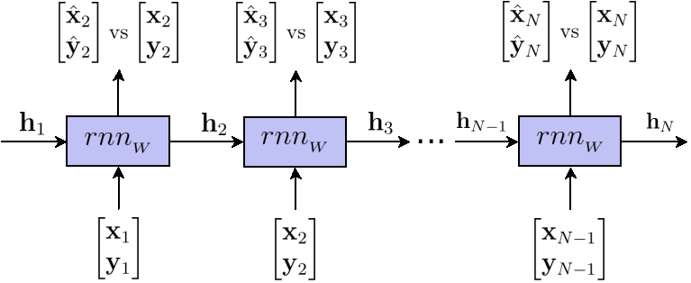
That is all a RNN is: a regular neural network that carries along a hidden state. It is trained the same way: by minimizing $MSE(\mathcal{\hat{Y}},\mathcal{Y})$ using gradient descent.
Long short-term memory (LSTM) models
By now, I emphasized multiple times how we don’t care about the internals of the neural network. That is partly because nowadays, the presented RNN equations have been superseded by a slightly more complex set of equations that form the base for the so-called “long short-term memory” (LSTM) models.
LSTMs present a RNN interface, but with different internals that provide them superior ability to remember or forget relevant pieces of information about the sequences being modelled, even when those pieces are far apart from each others within the input sequence (long range dependencies).
Let’s make the last statement more concrete by taking a face drawing as example:

In order to generate such a drawing, the neural network needs to know how to draw a circle. Most importantly, it need to know how to end drawing it where it started (long-range dependency between the first and last point of the circle). It then has to mostly forget about the circular shape, and focus on the eyes and the mouth, while retaining information about their relative position with respect to the enclosing circle. That is where vanilla RNNs fail and LSTMs shine.
In the rest of this post, I will abusively refer to LSTMs as just “RNNs”. They are indeed the de facto RNN models for any machine learning practitioner attempting to model sequences.
To be honest, it still blows my mind that a few thousand weights can hold such high-level information, and that a few matrix multiplication is enough to apply it.
Welcome to deep learning.
Diving into the inner workings of LSTMs is also out of the scope of this article, but the following article — widely cited, and deservedly so — should satisfy the curiosity of the interested reader.
Fist generated drawings
There is good news! We have finally everything we need to generate our first drawings.
For each category mentioned earlier (Eiffel tower, faces and fire truck), let’s grab a RNN, feed it ~11.000 drawings $\mathcal{X}$, output predictions $\mathcal{\hat Y}$, score them against the labels $\mathcal{Y}$ using the MSE, let the gradients flow back through the network, update the weights applying gradient descent, repeat multiple times (around 200 to 300 epochs) and, after half an hour of training per model on GPU …
Tada!!!
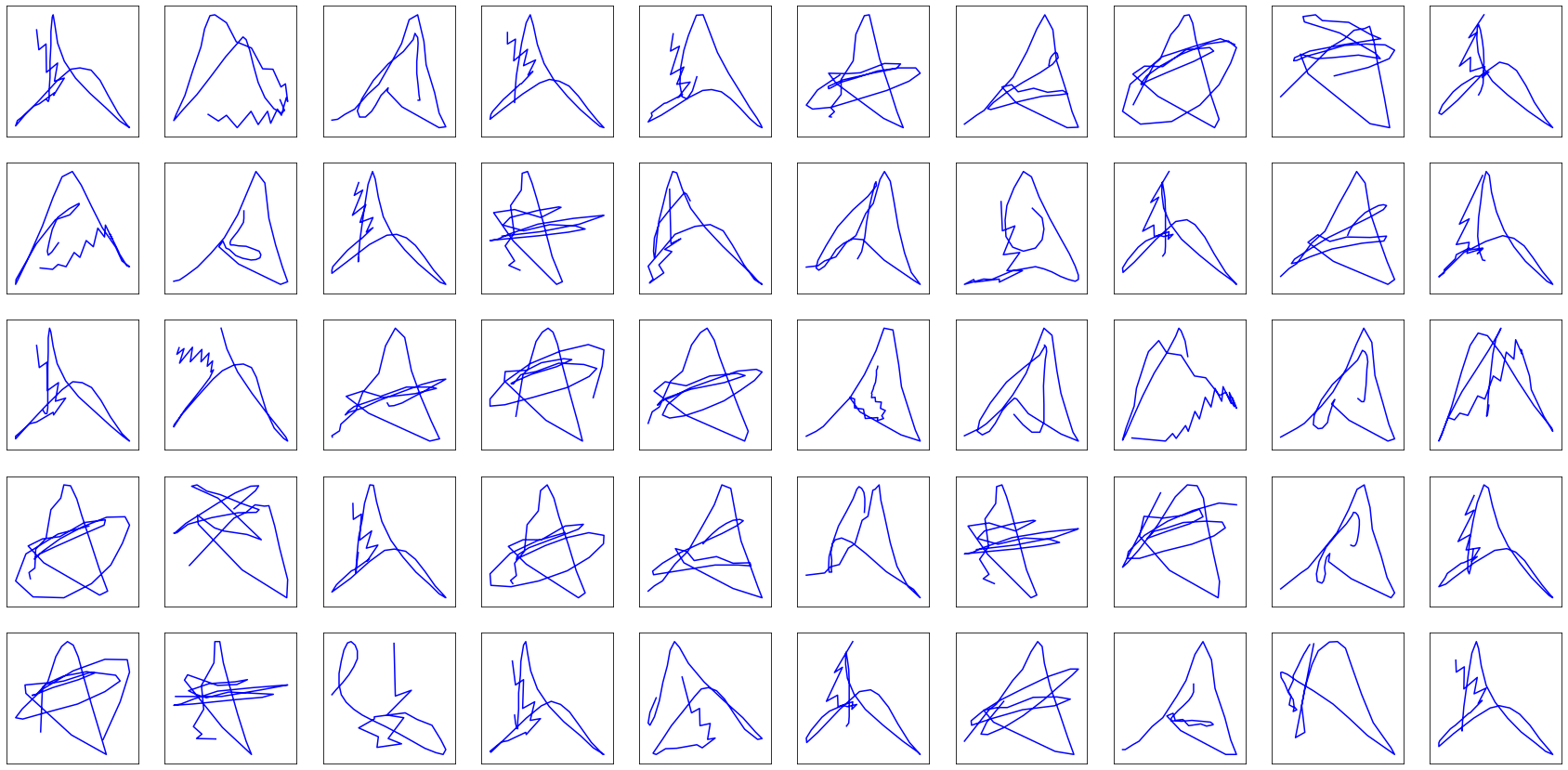
Pretty disappointing, right?
Well, not quite. At least the model identified the primitive shape of each class: the Eiffel towers are triangle-shaped, circles somewhat start to appear in faces, and upon closer inspection, you might distinguish rectangles in the generated fire truck drawings.
Before we find a way of improving the drawings trajectory, let’s focus on a more immediate problem: the model is unable to decide when to lift the pencil to start a new stroke, left alone when to stop drawing. For its defence, it is not its fault. We simply didn’t teach it how to.

The previous generated drawings have been limited to 25 points in order not to get out of hand.
Stroke state of drawings
I wrote earlier that drawings are represented in the dataset as sequences of vectors, and proceeded to represent a drawing as a contiguous sequence. But did I mention anywhere that the sequence had to be contiguous?
Since I value your sanity (and mine), let’s consider a simple drawing as example, and omit the initial $\overrightarrow 0$ vector. It will save us the indices nightmare.

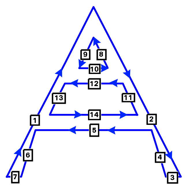
That fake Eiffel tower would be represented in the dataset as a list of three strokes between which the pencil is lifted $\mathcal{X} = \mathcal{S}_1,~\mathcal{S}_2,~\mathcal{S}_3$.
$$ \mathcal{S}_1 = \mathcal{X}_{1}~...~\mathcal{X}_{7}~~~~~~~~~~~ \mathcal{S}_2 = \mathcal{X}_{8}~...~\mathcal{X}_{10}~~~~~~~~~~~ \mathcal{S}_3 = \mathcal{X}_{11}~...~\mathcal{X}_{14} $$
While this shape of data is satisfying in terms of representational power, it is much less so in terms of model input. Indeed, a recurrent neural network expects a potentially variable length sequences of points as input, not variable-length sequences of variable-length sequences of points.
So we will have to flatten this representation somehow.
We already went done the most naive way, concatenating all strokes as one big stroke, and it did not go too well:
$$ \mathcal{X} = \begin{bmatrix} \mathbf{x}_1 ~~ ... ~~ \mathbf{x}_7 ~~ \mathbf{x}_8 ~~ ... ~~ \mathbf{x}_{10} ~~ \mathbf{x}_{11} ~~ ... ~~ \mathbf{x}_{14} \\ \mathbf{y}_1 ~~ ... ~~ \mathbf{y}_7 ~~ \mathbf{y}_8 ~~ ... ~~ \mathbf{y}_{10} ~~ \mathbf{y}_{11} ~~ ... ~~ \mathbf{y}_{14} \end{bmatrix} $$

So let’s try to insert a special value $\mathbf{\delta}$ between each stroke to inform the model where the pencil should be lifted. $\mathbf{\delta}$ should be big enough in absolute value so that is does not conflict with regular points components.
$$ \mathcal{X} = \begin{bmatrix} \mathbf{x}_1 ~~ ... ~~ \mathbf{x}_7 ~~ \mathbf{\delta} ~~ \mathbf{x}_8 ~~ ... ~~ \mathbf{x}_{10} ~~ \mathbf{\delta} ~~ \mathbf{x}_{11} ~~ ... ~~ \mathbf{x}_{14} \\ \mathbf{y}_1 ~~ ... ~~ \mathbf{y}_7 ~~ \mathbf{\delta} ~~ \mathbf{y}_8 ~~ ... ~~ \mathbf{y}_{10} ~~ \mathbf{\delta} ~~ \mathbf{y}_{11} ~~ ... ~~ \mathbf{y}_{14} \end{bmatrix} $$
That could potentially work, but the weird non-continuous behaviour introduced would almost certainly confuse the model. Moreover, how are we supposed to deal with the model output when it predicts $\delta$ on one dimension, but a regular value on the other one? That sounds like a source of endless complication.
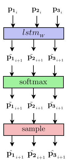
We would be better off selecting a third and last approach: introducing an input dimension $\mathbf{p_2}$ that signals the end of a stroke. While we’re at it, let’s use another dimension $\mathbf{p_3}$ to indicate the end of the drawing, and set $\mathbf{p_2} = 0$ when that occurs. Finally, since it is nice to have all additional dimensions summing to 1, let’s intercalate the complementary “regular point” dimension $\mathbf{p_3}$, better described as “neither end of stroke nor end of drawing”:
$$ \mathcal{X} = \begin{bmatrix} \mathbf{x}_1 & ... & \mathbf{x}_7 & \mathbf{x}_8 & ... & \mathbf{x}_{10} & \mathbf{x}_{11} & ... & \mathbf{x}_{14} \\ \mathbf{y}_1 & ... & \mathbf{y}_7 & \mathbf{y}_8 & ... & \mathbf{y}_{10} & \mathbf{y}_{11} & ... & \mathbf{y}_{14} \\ 1 & 1 & 0 & 1 & 1 & 0 & 1 & 1 & 0 \\ 0 & 0 & 1 & 0 & 0 & 1 & 0 & 0 & 0 \\ 0 & 0 & 0 & 0 & 0 & 0 & 0 & 0 & 1 \end{bmatrix} \begin{matrix} \\ \\ \leftarrow\footnotesize{\mathbf{p_1}\text{: is regular point?~~~~~~~~~~~~~~}} \\ \leftarrow\footnotesize{\mathbf{p_2}\text{: is end-of-stroke point?~~~}} \\ \leftarrow\footnotesize{\mathbf{p_3}\text{: is end-of-drawing point?}} \end{matrix} $$
We name $\begin{bmatrix} \mathbf{x}_i,~\mathbf{y}_i \end{bmatrix}$ the trajectory and $\begin{bmatrix} \mathbf{p_1}_i,~\mathbf{p_2}_i,~\mathbf{p_3}_i \end{bmatrix}$ the stroke state.
A joint regression and classification model
Modelling the trajectory is a regression problem with real-valued labels $\begin{bmatrix} \mathbf{x}_{i+1},~\mathbf{y}_{+1} \end{bmatrix}$, and modelling the stroke state a classification problem with labels $\begin{bmatrix} \mathbf{p_1}_{i+1},~\mathbf{p_2}_{i+1},~\mathbf{p_3}_{i+1} \end{bmatrix}$ that pertain to one of three classes: regular point $\begin{bmatrix} 1, 0, 0 \end{bmatrix}$, end of stroke $\begin{bmatrix} 0, 1, 0 \end{bmatrix}$ or end of drawing $\begin{bmatrix} 0, 0, 1 \end{bmatrix}$.
Our model solves both jointly. It takes as input 5-dimensional vectors
$\mathcal{X}_i = \begin{bmatrix} \mathbf{x}_i,~\mathbf{y}_i,~\mathbf{p_1}_i,~\mathbf{p_2}_i,~\mathbf{p_3}_i \end{bmatrix}$,
output similarly shaped predictions
$\mathcal{\hat Y}_i = \begin{bmatrix} \mathbf{\hat x}_{i+1},~\mathbf{\hat y}_{i+1},~\tilde{\mathbf{p_1}}_{i+1},~\tilde{\mathbf{p_2}}_{i+1},~\tilde{\mathbf{p_3}}_{i+1} \end{bmatrix}$, and score them against labels
$\mathcal{Y}_i = \begin{bmatrix} \mathbf{x}_{i+1},~\mathbf{y}_{i+1},
\mathbf{p_1}_{i+1},~\mathbf{p_2}_{i+1},~\mathbf{p_3}_{i+1} \end{bmatrix}$ using the 5-dimensional $MSE$:
$$ \begin{aligned} MSE&(\mathcal{\hat{Y}},\mathcal{Y})= \frac{1}{N}\sum_{i=1}^N (\mathbf{\hat{x}}_{i+1} - \mathbf{x}_{i+1}) ^ 2 + (\mathbf{\hat{y}}_{i+1} - \mathbf{y}_{i+1}) ^ 2~+ \\ &+ \frac{1}{N}\sum_{i=1}^N (\tilde{\mathbf{p_1}}_{i+1} - \mathbf{p_1}_{i+1}) ^ 2 + (\tilde{\mathbf{p_2}}_{i+1} - \mathbf{p_2}_{i+1}) ^ 2 + (\tilde{\mathbf{p_3}}_{i+1} - \mathbf{p_3}_{i+1}) ^ 2 \end{aligned} $$
At this point, the reader accustomed to fitting classification models may wonder “what’s this guy even doing? MSE as classification loss? Nobody does that”. Sure, but can you name the flawed assumption we are making when doing so? If you’re thinking likelihood of some normal distribution, you’re on the right path. If not, that is a question the article will clearly answer later on. For the time being, please accept the MSE.
Generating the stroke state
There is a more pressing issue: the model outputs $\begin{bmatrix} \tilde{\mathbf{p_1}}_{i+1},~\tilde{\mathbf{p_2}}_{i+1},~\tilde{\mathbf{p_3}}_{i+1} \end{bmatrix}$ are abritrary numbers, not valid stroke states, for which one component equals $1$ while the others are $0$. Sure, we could force this property by making the highest component go to $1$ and the others to $0$, but it would result in a non-derivable model incompatible with gradient descent. Instead, let’s introduce a much smarter idea.
First, let’s normalize each model output using a softmax function (detailed below), so that $\tilde{\mathbf{p_1}}_{i+1} + \tilde{\mathbf{p_2}}_{i+1} + \tilde{\mathbf{p_3}}_{i+1} = 1$. Second, let’s consider these numbers define a probability mass function for a discrete probability distribution. Finally, let’s sample the real stroke state predictions from the distribution, as such:
- Draw “regular point” event $\hat{\mathcal{Y}}_i = \begin{bmatrix} 1,0,0 \end{bmatrix}$ with probability $\tilde{\mathbf{p_{1}}}_{i+1}$
- Draw “end of stroke” event $\hat{\mathcal{Y}}_i = \begin{bmatrix} 0,1,0 \end{bmatrix}$ with probability $\tilde{\mathbf{p_{2}}}_{i+1}$
- Draw “end of drawing” event $\hat{\mathcal{Y}}_i = \begin{bmatrix} 0,0,1 \end{bmatrix}$ with probability $\tilde{\mathbf{p_{3}}}_{i+1}$
That is the first occurence of a probabilistic layer on top of the RNN. Congratulations, you have made it to the second half of the article. Please take good note of the difference in notation between the model outputs $\tilde{\mathbf{p_k}}_{i+1}$ using a tilde $\tilde ~$, and the actual stroke state predictions using a hat $\hat ~$.
leaving the trajectory and hidden state aside.
Normalizing model outputs
Temporarily getting rid of the annoying $_{i+1}$ indices, the most obvious form of normalization for the model outputs is as follows:
$$ \text{normalize}(\tilde{\mathbf{p_k}}) = \frac{\tilde{\mathbf{p_k}}}{\sum\limits_{k=1}^3 \tilde{\mathbf{p_k}}},~~k=1..3 $$
We are going to a more flexible version:
$$ \text{softmax}_{_{T_\mathbf{p}}}(\tilde{\mathbf{p_k}}) = \frac{\exp(\tilde{\mathbf{p_k}}~/~T_\mathbf{p})}{\sum\limits_{k=1}^3 \exp(\tilde{\mathbf{p_k}}~/~T_\mathbf{p})},~~k=1..3 $$
$T_\mathbf{p}$ is a generation parameter called temperature. It defines how inclined the softmax is at giving importance to lower $\tilde{\mathbf{p_k}}$’s. Since it can be conceptually difficult to gauge the influence of $T_\mathbf{p}$ from the equation alone, let’s visualize it.
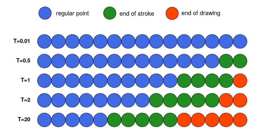
for model outputs $\begin{bmatrix} \tilde{\mathbf{p_1}}_{i+1},~\tilde{\mathbf{p_2}}_{i+1},~\tilde{\mathbf{p_3}}_{i+1} \end{bmatrix} = \begin{bmatrix} 3, 2, 1 \end{bmatrix}$.
Or more concretely with actual Eiffel towers generation:
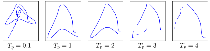
At low temperature ($T_\mathbf{p} = 0.1$), the model does not take any risk and consistently outputs the stroke state most represented in the data: regular point $\begin{bmatrix} 1,~0,~0 \end{bmatrix}$, thus ending up with drawings that continue indefinitely without lifting the pencil once, much like our former trajectory-only model. When temperature goes up, the model dares sampling more and more of the other stroke states, making the drawings more fragmented (more end-of-stroke points $\begin{bmatrix} 0,~1,~0 \end{bmatrix}$) and shorter (higher probability of eventually generating end-of-drawing event $\begin{bmatrix} 0,~0,~1 \end{bmatrix}$).
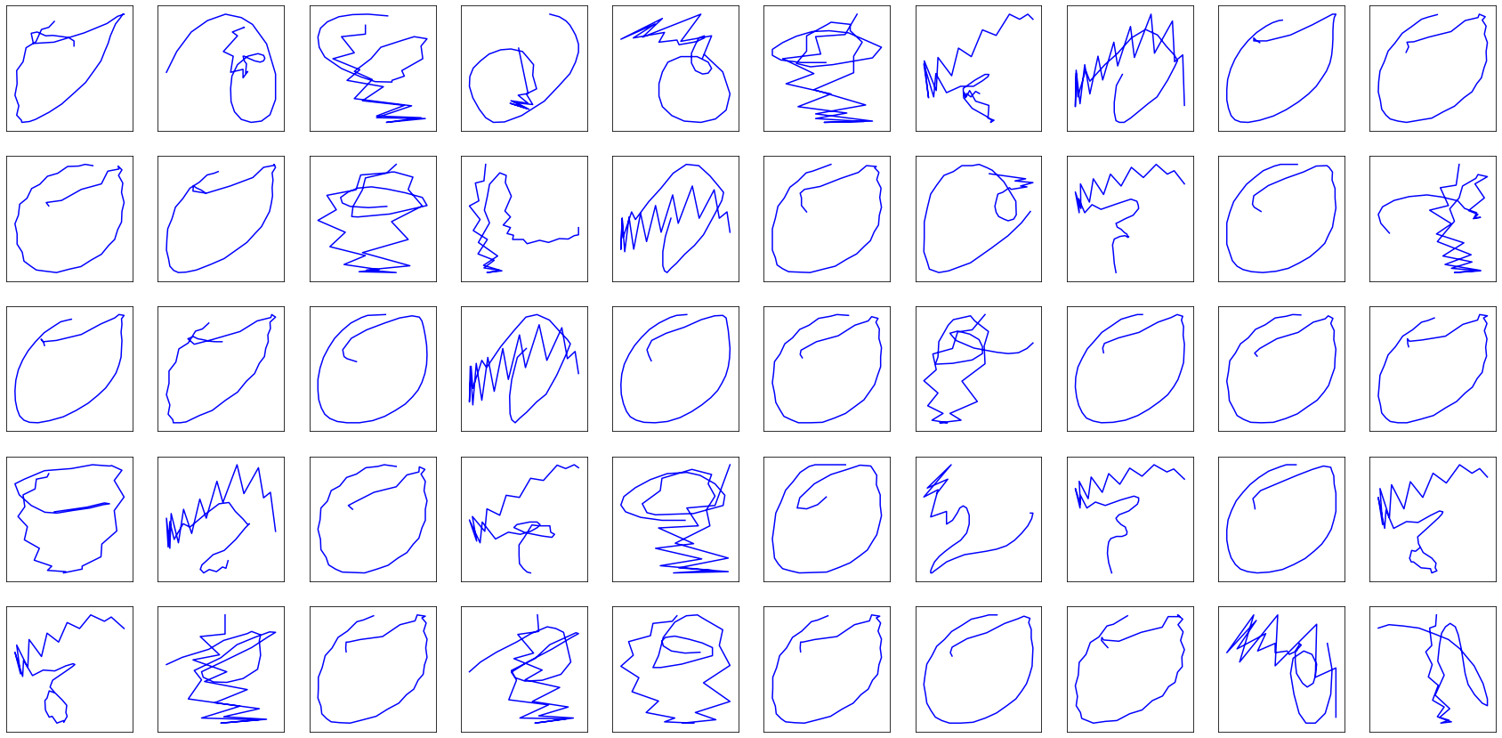
Second generated drawings
By now, the model can lift pencil and stop drawing by itself. Let’s train it with $T_\mathbf{p}=1$ — as will always be the case, $T_\mathbf{p}$ being a generation parameter only — and generate some some drawings with $T_\mathbf{p} = 0.8$:

Hey! The generated Eiffel towers and faces are starting to look like ones. The fire trucks are still pretty disappointing, most likely owning it to disastrous trajectory predictions rather than stroke state predictions. They will hopefully get better as we push further the idea of turning our LSTM from yet-too-deterministic to fully probabilistic.
Making the model probabilistic
Trajectory as a random variable
Let’s put the stroke state aside for one moment, and consider how the trajectory $\mathcal{X}_i = \begin{bmatrix} \mathbf{x}_{i},~\mathbf{y}_{i} \end{bmatrix}$ is modelled.
Currently, ignoring the hidden state, the model deterministically outputs a prediction for the next vector:
$$ \mathcal{\hat{Y}_i} = lstm_{_W}(\mathcal{X_i}) $$
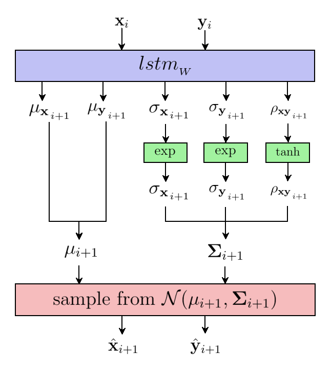
Guess what? We are going to apply the same idea as for the stroke state. Instead of directly predicting the next vector $\hat{\mathcal{Y}}_i$, let’s have the model output a 5-dimensional vector $\tilde{\mathcal{Y}}_i$:
$$ \mathcal{\tilde{Y}_i} = \begin{bmatrix} \mathbf{\mu_x}_{_{i+1}},~\mathbf{\mu_y}_{_{i+1}},~\mathbf{\sigma_x}_{_{i+1}},~\mathbf{\sigma_y}_{_{i+1}},~\mathbf{\rho_{xy}}_{_{i+1}} \end{bmatrix} = lstm_{_W}(\mathcal{X_i}) $$
In order to make the next equations a little tidier, let’s temporarily omit the annoying $_{i+1}$ indices by setting $\mathcal{\tilde{Y}_i} = \begin{bmatrix} \mu_x,~\mu_x,~\sigma_x,~\sigma_y,~\rho_{xy} \end{bmatrix}$.
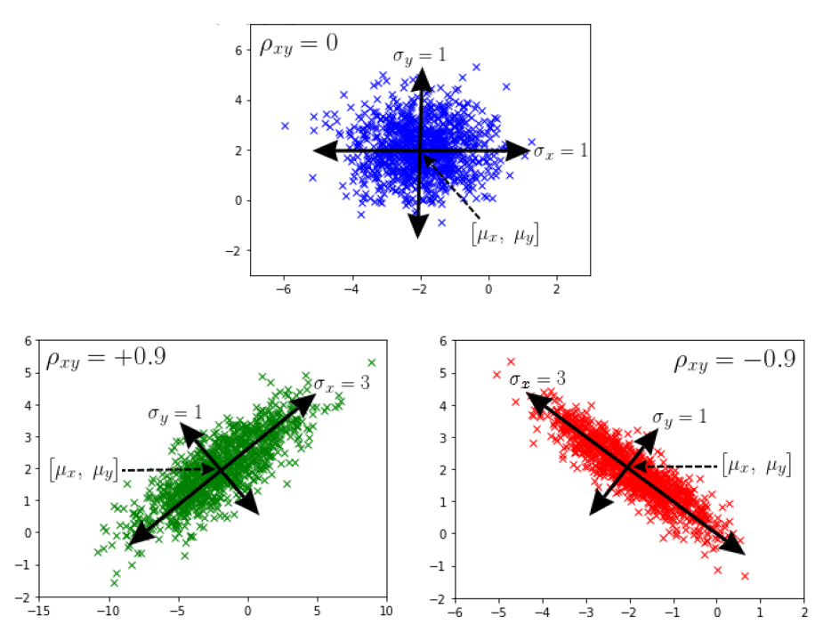
You may recognize these symbols. They are the parameters of a 2-dimensional normal distribution:
- $\begin{bmatrix} \mu_x,~\mu_y \end{bmatrix}$ is the center of the distribution.
- $\sigma_x$ and $\sigma_y$ are the variances in the direction of x and y, both greater than 0.
- $\rho_{xy}$ is the correlation coefficient between x and y, ranging between -1 and 1 (excluded).
In particular, when $\mathbf{\rho_{xy}} = 0$, the distribution is equivalent to two independent normals along x and y.
Much like we enforced $\tilde{\mathbf{p_1}} + \tilde{\mathbf{p_2}} + \tilde{\mathbf{p_3}} = 1$ for the output stroke state, we can make sure that $\mathbf{\sigma_x}$ and $\mathbf{\sigma_y}$ are greater than 0 by passing them through an exponential, and that $\mathbf{\rho_{xy}}$ is between -1 and 1 by passing it through a hyperbolic tangent.
Finally, the actual prediction for the next vector $\hat{\mathcal{Y}}_i = \begin{bmatrix} \hat{\mathbf{x}}_{i+1},~\hat{\mathbf{y}}_{i+1} \end{bmatrix}$ is sampled from the normal $\mathcal{N}(\mathbf{\mu}_{i+1}, \mathbf{\Sigma}_{i+1})$ centered at $\mathbf{\mu}_{i+1} = \begin{bmatrix} \mu_x,~\mu_y \end{bmatrix}$ with covariance matrix $\Sigma_{i+1} = \begin{bmatrix} \sigma_x^2 & \rho_{xy} \sigma_x \sigma_y \\ \rho_{xy} \sigma_x \sigma_y & \sigma_x^2 \end{bmatrix}$.
leaving the stroke state and hidden state aside.
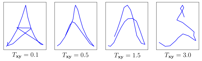
It order to gain the same flexibility for trajectory generation as we had for stroke state generation, let’s scale the spread of the distribution by a temperature parameter $T_\mathbf{xy}$ by setting $\mathbf{\Sigma}_{i+1} = T_\mathbf{xy} \times \mathbf{\Sigma}_{i+1}$. The temperature determines how far from the center $\mathbf{\mu}_{i+1}$ the model is allowed to sample $\mathcal{\hat{Y}_i}$. When $T_\mathbf{xy} \to 0$, we end up with a model resembling our former deterministic model, consistently outputting $\begin{bmatrix} \mathbf{\mu_{x}},~\mathbf{\mu_{y}} \end{bmatrix}$. When $T_\mathbf{xy} \to \infty$, we end up with fully random trajectories.
Taking a leap into the future, let’s attempt to generate Eiffel towers at various temperatures. The highest the temperature, the most chaotic the trajectory.
Great! We now have a probabilistic model for both trajectory and stroke state generation.
Training trajectory
The battle is not over, though. We still have to train the model. While we cowardly got away with the MSE for the stroke state, good luck applying it to 5-dimensional trajectory outputs and incompatible labels of dimension 2.
More seriously, how do we define a loss $\mathscr{L}(\begin{bmatrix} \mathbf{\mu}_{i+1},~\mathbf{\Sigma}_{i+1} \end{bmatrix},~\mathcal{Y}_i)$ that quantifies the adequacy of the model outputs with their corresponding labels?
It turns out probability theory provides a neat answer to that question: just use the density $p_{\mathbf{\mu}_{i+1},~\mathbf{\Sigma}_{i+1}}$ of normal distribution $\mathcal{N}(\mathbf{\mu}_{i+1}, \mathbf{\Sigma}_{i+1})$:
$$ p_{\mathbf{\mu},~\mathbf{\Sigma}}(x, y) = \frac{1}{2 \pi \mathbf{\sigma_x} \mathbf{\sigma_y} \sqrt{1-\mathbf{\rho_{xy}}^2}} \exp\left( -\frac{1}{2(1-\mathbf{\rho_{xy}}^2)}\left[ \frac{(x-\mathbf{\mu_x})^2}{\mathbf{\sigma_x}^2} +\frac{(y-\mathbf{\mu_y})^2}{\mathbf{\sigma_y}^2} -\frac{2\mathbf{\rho_{xy}}(x-\mathbf{\mu_y})(y-\mathbf{\mu_y})}{\mathbf{\sigma_x} \mathbf{\sigma_y}} \right] \right) $$
By the very definition of continuous probability distribution, the larger the value of $p_{\mathbf{\mu}_{i+1},~\mathbf{\Sigma}_{i+1}}(\mathcal{Y}_i)$, the better the chance of sampling $\mathcal{Y}_i$ from $\mathcal{N}(\mathbf{\mu}_{i+1},~\mathbf{\Sigma}_{i+1})$. While it is relevant for generation, it is not for training. Taking it backward, however, the higher the value of $p_{\mathbf{\mu}_{i+1},~\mathbf{\Sigma}_{i+1}}(\mathcal{Y}_i)$, the better the chance — precisely, the likelihood — that model output $\mathbf{\mu}_{i+1},~\mathbf{\Sigma}_{i+1}$ form a normal $\mathcal{N}(\mathbf{\mu}_{i+1},~\mathbf{\Sigma}_{i+1})$ from which label $\mathcal{\mathcal{Y}_i}$ could have been sampled.
The concept is easily generalized to all labels $\mathcal{Y} = \mathcal{Y}_1,~…,~\mathcal{Y}_N$ and models outputs $\tilde{\mathcal{Y}} = \begin{bmatrix} \mathbf{\mu}_1,~\mathbf{\Sigma}_1 \end{bmatrix}, …, \begin{bmatrix} \mathbf{\mu}_N,~\mathbf{\Sigma}_N \end{bmatrix}$ by defining the likelihood function:
$$ \mathcal{L}(\mathcal{Y}~;~\mu, \mathbf{\Sigma}) = \prod_{i=1}^N p_{\mathbf{\mu}_{i+1},~\mathbf{\Sigma}_{i+1}}(\mathcal{Y}_i) $$
At this point, we’re almost done. Indeed, maximizing this quantity (a process known as maximum likelihood estimation) effectively maximizes the adequacy of the model outputs to the labels, assuming independence of the $\mathcal{Y}_i$’s,.
However, since we much prefer means to products for reasons of numerical stability, and $\argmin$ to $\argmax$ in order to define a loss, please consider the two following properties of $\argmax$:
- wrapping what’s inside $\argmax$ into whatever strictly increasing function (such as $\log$) does not change the value of the $\argmax$.
- maximizing a function is the same as minimizing its opposite: $\argmax f = \argmin -f$.
So:
$$ \begin{aligned} W_{optimal} =~& \underset{W}{\argmax} \prod_{i=1}^N p_{\mathbf{\mu}_{i+1},~\mathbf{\Sigma}_{i+1}}(\mathcal{Y}_i) \\ \underset{\log}{=}~& \underset{W}{\argmax}~ \log \left( \prod_{i=1}^N p_{\mathbf{\mu}_{i+1},~\mathbf{\Sigma}_{i+1}}(\mathcal{Y}_i) \right) \\ =~& \underset{W}{\argmax} \sum_{i=1}^N \log p_{\mathbf{\mu}_{i+1},~\mathbf{\Sigma}_{i+1}}(\mathcal{Y}_i) \\ \underset{\times \frac{1}{N}}{=}~& \underset{W}{\argmax} \frac{1}{N} \sum_{i=1}^N \log p_{\mathbf{\mu}_{i+1},~\mathbf{\Sigma}_{i+1}}(\mathcal{Y}_i) \\ W_{optimal} \underset{\times \text{-}1}{=}~& \underset{W}{\argmin} - \frac{1}{N} \sum_{i=1}^N \log p_{\mathbf{\mu}_{i+1},~\mathbf{\Sigma}_{i+1}}(\mathcal{Y}_i) \end{aligned} $$
We’re left with the minimization of a function with respect to its parameters given the labels and model. Does that ring a bell?
It is a loss function!
Victory!
Omitting the hidden state:
$$ \mathscr{L}_{\text{trajectory}}(\tilde{\mathcal{Y}},\mathcal{Y}) = -\frac{1}{N} \sum_{i=1}^N \log p_{\mathbf{\mu}_{i+1},~\mathbf{\Sigma}_{i+1}}(\mathcal{Y}_i) \\[5pt] \text{where } \tilde{\mathcal{Y}} = \begin{bmatrix} \mathbf{\mu},~\mathbf{\Sigma} \end{bmatrix} = lstm_{_W}(\mathcal{X}) $$
Or, replacing $p_{\mathbf{\mu}_{i+1},~\mathbf{\Sigma}_{i+1}}$ with its actual equation:
$$ \begin{aligned} \mathscr{L}_{\text{trajectory}}(\tilde{\mathcal{Y}},\mathcal{Y}) =& -\frac{1}{N}\sum_{i=1}^N log(2 \pi \mathbf{\sigma_x}_{_{i+1}} \mathbf{\sigma_y}_{_{i+1}} \sqrt{1-\mathbf{\rho_{xy}}_{_{i+1}}^2}) \\ &+ \frac{1}{N}\sum_{i=1}^N \frac{1}{2 (1 - \mathbf{\rho_{xy}}_{_{i+1}}^2)} \left[ \frac{(\mathbf{x}_{i+1}-\mathbf{\mu_x}_{_{i+1}})^2}{\mathbf{\sigma_x}_{_{i+1}}^2} + \frac{(\mathbf{y}_{i+1}-\mathbf{\mu_y}_{_{i+1}})^2}{\mathbf{\sigma_y}_{_{i+1}}^2} \right] \\ &-\frac{1}{N}\sum_{i=1}^N \frac{\mathbf{\rho_{xy}}_{_{i+1}}(\mathbf{x}_{i+1}-\mathbf{\mu_x}_{_{i+1}})(\mathbf{y}_{i+1}-\mathbf{\mu_y}_{_{i+1}})} {(1 - \mathbf{\rho_{xy}}_{_{i+1}}^2)~\mathbf{\sigma_x}_{_{i+1}} \mathbf{\sigma_y}_{_{i+1}}} \end{aligned} \\[5pt] \text{where } \begin{bmatrix} \mathbf{\mu_x}_{_{i+1}},~\mathbf{\mu_y}_{_{i+1}},~\mathbf{\sigma_x}_{_{i+1}},~\mathbf{\sigma_{y}}_{_{i+1}},~\mathbf{\rho_{xy}}_{_{i+1}} \end{bmatrix} = lstm_{_W}(\mathcal{X}_i) $$
Ouch. Sorry for that one.
The new loss is rather scary, especially as compared to our previous MSE. But now, not only are we optimizing the center of the predictions $\mathbf{\mu}_{i+1}$, we are also optimizing their variance $\mathbf{\Sigma}_{i+1}$.
In fact, the MSE is a special case of that loss, and clarifying in what way provides valuable insight.
The hidden assumptions of MSE
Let’s assume independent normal distributions ($\mathbf{\rho_{xy}} = 0$) and equal variance ($\sigma_x = \sigma_y = \sigma$) along x and y across all model outputs. We end up with an isotropic covariance matrices $\Sigma = \begin{bmatrix} \mathbf{\sigma}^2 & 0 \\ 0 & \mathbf{\sigma}^2 \end{bmatrix}$ and the following loss:
$$ \mathscr{L}_{\text{trajectory}}(\tilde{\mathcal{Y}},~\mathcal{Y}) = \frac{1}{N}\sum_{i=1}^N log(2 \pi) + \frac{1}{\sigma} \left[ (\mathbf{x}_{i+1} - \mathbf{\mu_x}_{_{i+1}})^2 + (\mathbf{y}_{i+1} - \mathbf{\mu_y}_{_{i+1}})^2 \right] \\[5pt] \text{where } \tilde{\mathcal{Y}}_i = \begin{bmatrix} \mathbf{\mu_x}_{_{i+1}},~\mathbf{\mu_y}_{_{i+1}} \end{bmatrix} = lstm_{_W}(\mathcal{X_i}) $$
Since we are minimizing $\mathscr{L}(\mathcal{\hat{Y}},\mathcal{Y})$, the constant terms $log(2 \pi)$ and $\frac{1}{\sigma}$ can be safely removed. Furthermore, assuming the predictions are directly the centers outputted by the model ($\hat{\mathcal{Y}} = \tilde{\mathcal{Y}}$):
$$ \begin{aligned} &\mathscr{L}_{\text{trajectory}}(\mathcal{\hat{Y}},\mathcal{Y}) = \frac{1}{N}\sum_{i=1}^N (\mathbf{x}_{i+1} - \hat{\mathbf{x}}_{i+1})^2 + (\mathbf{y}_{i+1} - \hat{\mathbf{y}}_{i+1})^2 \\ &\mathscr{L}_{\text{trajectory}}(\mathcal{\hat{Y}},\mathcal{Y}) = MSE(\mathcal{\hat{Y}},\mathcal{Y}) \end{aligned} $$
We’re coming full circle, but with a fundamental insight: the mean squared error is not just a random loss. It has a more profound meaning: minimizing the MSE between the predictions and the labels is equivalent to maximizing the likelihood of the labels under a normal distribution with isotropic covariance matrix.
Stroke state training
Let’s now apply the same principles as in the last section to derive an adequate loss function for the stroke state.
We previously used MSE as loss, and I challenged you to tell why it wasn’t a good idea. The last section provides a neat answer to that question: it assume a normal distribution over the stroke states.
Does it seem like a reasonable assumption for a set of three possible events?
Nop.
The actual stroke state distribution is much simpler than that. Leaving trajectory aside, the output of the model $\tilde{\mathcal{Y}}_{i} = \tilde{\mathbf{p}}_{i+1} = \begin{bmatrix} \tilde{\mathbf{p_1}}_{i+1},~\tilde{\mathbf{p_2}}_{i+1},~\tilde{\mathbf{p_3}}_{i+1} \end{bmatrix}$ defines a probability mass function $p_{\tilde{\mathbf{p}}_{i+1}}$ (the equivalent of the density function, but for discrete distributions) over the three possible stroke states, which can be evaluated against the corresponding label $\mathcal{Y}_{i} = \begin{bmatrix} \mathbf{p_1}_{i+1},~\mathbf{p_2}_{i+1},~\mathbf{p_3}_{i+1} \end{bmatrix}$ in a straightforward manner:
$$ p_{\tilde{\mathbf{p}}_{i+1}}(\mathcal{Y}_i) = \begin{cases} {\tilde{\mathbf{p_1}}_{i+1}} \text{ if } \mathcal{Y}_i = \begin{bmatrix} 1,0,0 \end{bmatrix} \\ {\tilde{\mathbf{p_2}}_{i+1}} \text{ if } \mathcal{Y}_i = \begin{bmatrix} 0,1,0 \end{bmatrix} \\ {\tilde{\mathbf{p_3}}_{i+1}} \text{ if } \mathcal{Y}_i = \begin{bmatrix} 0,0,1 \end{bmatrix} \end{cases} $$
In plain English, $p_{\tilde{\mathbf{p}}_{i+1}}(\mathcal{Y}_i)$ is the probability outputted by the model for the correct class. The higher, the better.
It can be pleasantly rewritten as:
$$ p_{\tilde{\mathbf{p}}_{i+1}}(\mathcal{Y}_i) = \prod_{k=1}^3 \tilde{\mathbf{p_k}}_{i+1}^{\mathbf{p_k}_{i+1}} $$
By the same derivation as for the trajectory, assuming independance of the $\mathcal{Y}_i$’s, we end up with a loss as standard as the MSE, but for classification. It is the cross-entropy loss:
$$ \begin{aligned} \mathscr{L}_{\text{stroke state}}(\tilde{\mathcal{Y}}, \mathcal{Y}) =& - \frac{1}{N} \sum_{i=1}^N \log(p_{\tilde{\mathbf{p}}_{i+1}}(\mathcal{Y}_i)) \\ =& - \frac{1}{N} \sum_{i=1}^N \sum_{k=1}^3 \mathbf{p_k}_{i+1} \log \tilde{\mathbf{p_k}}_{i+1} \end{aligned} $$
Third generated drawings
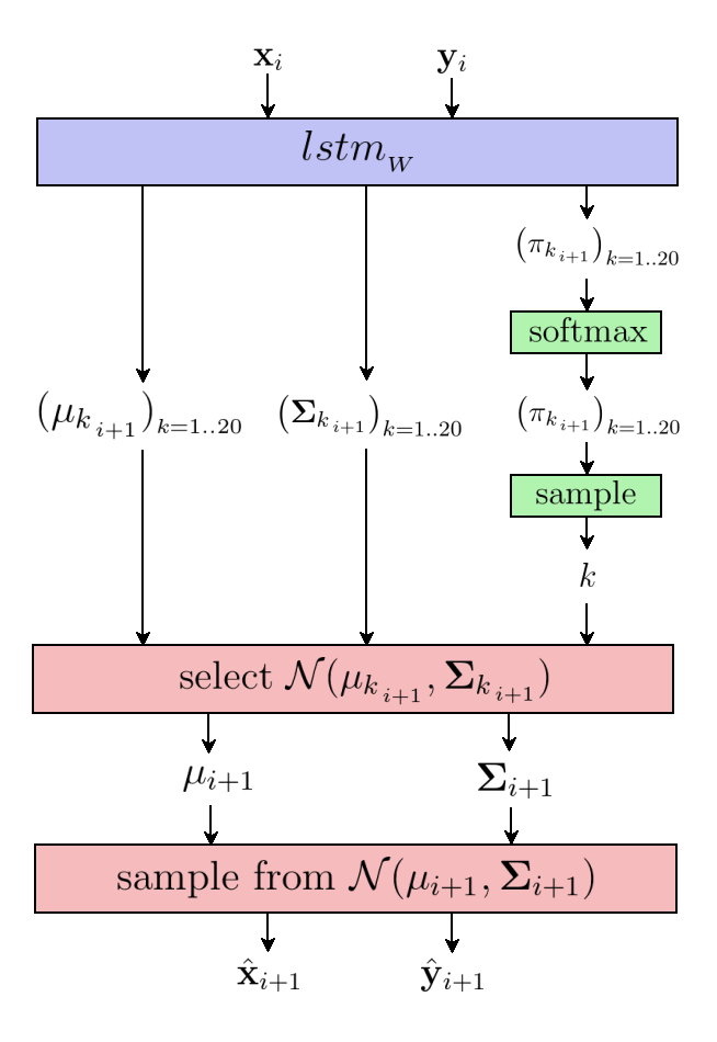
Putting it all together, we are left with a RNN that takes 5 number
$\mathcal{X}_i = \begin{bmatrix} \mathbf{x}_i,~\mathbf{y}_i,~\mathbf{p_1}_i,~\mathbf{p_2}_i,~\mathbf{p_3}_i \end{bmatrix}$
and a hidden state vector $\mathbf{h}_i$ of size $H = 128$ as
input, and outputs 8 numbers
$\tilde{\mathcal{Y}}_i = \begin{bmatrix} \mathbf{\mu_x}_{_{i+1}},~\mathbf{\mu_y}_{_{i+1}},~\mathbf{\sigma_x}_{_{i+1}},~\mathbf{\sigma_y}_{_{i+1}},~\mathbf{\rho_{xy}}_{_{i+1}},~\tilde{\mathbf{p_1}}_{_{i+1}},~\tilde{\mathbf{p_2}}_{_{i+1}},~\tilde{\mathbf{p_3}}_{_{i+1}}
\end{bmatrix}$
and a hidden state vector $\mathbf{h}_{i+1}$:
$$ \tilde{\mathcal{Y}}_i,~\mathbf{h}_{i+1} = lstm_{_W}(\mathcal{X_i},~ \mathbf{h}_i) $$
It is trained by matching its outputs against the corresponding labels $\mathcal{Y}_i = \begin{bmatrix} \mathbf{x}_{i+1},~\mathbf{y}_{i+1},~\mathbf{p_1}_{i+1},~\mathbf{p_2}_{i+1},~\mathbf{p_3}_{i+1} \end{bmatrix}$ using the half-regression half-classification loss:
$$ \begin{aligned} \mathscr{L}(\tilde{\mathcal{Y}},\mathcal{Y}) =&~ \mathscr{L}_{\text{trajectory}}(\tilde{\mathcal{Y}},\mathcal{Y}) + \mathscr{L}_{\text{stroke state}}(\tilde{\mathcal{Y}},\mathcal{Y}) \\ =& -\frac{1}{N} \sum_{i=1}^N \log p_{\mathbf{\mu}_{i+1},~\mathbf{\Sigma}_{i+1}(\mathcal{Y}_i)} ~~ -\frac{1}{N} \sum_{i=1}^N \log p_{\tilde{\mathbf{p}}_{i+1}(\mathcal{Y}_i)} \end{aligned} $$
Generation is achieved by sampling the next trajectory and stroke state $\hat{\mathcal{Y}}_i = \begin{bmatrix} \hat{\mathbf{x}}_{i+1},~\hat{\mathbf{y}}_{i+1},~\hat{\mathbf{p_1}}_{i+1},~\hat{\mathbf{p_2}}_{i+1},~\hat{\mathbf{p_3}}_{i+1} \end{bmatrix}$ from the resulting probability distributions at given temperatures $T_\mathbf{xy}$ and $T_\mathbf{p}$:
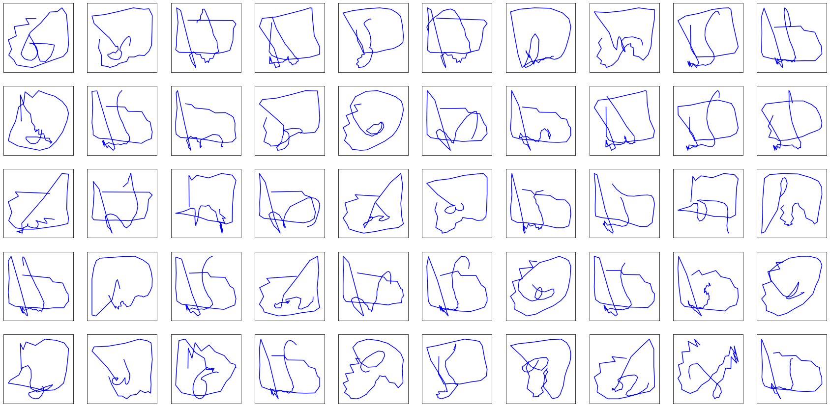
And finally, here come the results:
Ouch … Not quite as satisfying as expected after such a struggle. Sure, Eiffel towers and faces are getting more realistic, but fire trucks … Something must be definitely wrong with the model.
Actually, yes.
Luckily, the last piece of maths we need to make it right is quite a straightforward one, especially as compared to what we endured in the last paragraphs. We’re actually very close to tackling drawings generation for good. Let’s lose our sanity and upgrade the 5-parameters normal modelling the trajectory to one with 120 parameters.
Gaussian mixture models
As the motto of machine learning practitioners goes: “all models are wrong, but some are useful”. While our model is useful, it still does not get the trajectories right enough.
The reason is simple: we assumed a normal distribution for the trajectory, even though we saw it wasn’t the case when we plotted it at the beginning of the article (symmetric, but too spread out):
So let’s upgrade to a more sophisticated probability distribution. Instead of having the model return the parameters for a single normal, let’s have it return the parameters for $K$ of them: $K$ centers $({\mathbf{\mu_k}}_{_{i+1}}) _{k=1..K}$ and $K$ covariance matrices $({\mathbf{\Sigma_k}}_{_{i+1}}) _{k=1..K}$. On top of those, let’s add $K$ coefficients $({\mathbf{\pi_k}}_{_{i+1}}) _{k=1..20}$ associated with the normals, that we will force to satisfy $\sum_{k=1}^K {\mathbf{\pi_k}}_{_{i+1}} = 1$ by passing them through a softmax conditioned on the trajectory temperature $T_\mathbf{xy}$:
$$ {\mathbf{\pi_k}}_{_{i+1}} = \frac{\exp({\mathbf{\pi_k}}_{_{i+1}}~/~T_\mathbf{xy})}{\sum\limits_{k=1}^3 \exp({\mathbf{\pi_k}}_{_{i+1}}~/~T_\mathbf{xy})},~~k=1..K $$
Sampling goes as follows: pick up one of the $K$ normals $\mathcal{N}({\mathbf{\mu}_k}_{_{i+1}}, {\mathbf{\Sigma}_k}_{_{i+1}})$ with probability ${\mathbf{\pi_k}}_{_{i+1}}$ and sample from it. The resulting probability distribution is called a gaussian mixture model, or GMM.
As in the Google Brain paper, we’re going to use $K=20$ normals, resulting in the RNN outputting $K$ centers (2 numbers each), $K$ covariance matrices (3 numbers each) and $K$ coefficients (1 number each), for a total of $(2 + 3 + 1) \times K = 120$ outputs for each next point prediction.
As a last step, we have to derive a loss for the GMM-modelled trajectory. It turns out to be a pretty straightforward extension of the previous loss, given the density $p_{{\mathbf{\mu_k}}_{_{i+1}},~{\mathbf{\Sigma_k}}_{_{i+1}}}$ of the $k$-th normal for the $i$-th output:
$$ \mathscr{L}_{\text{trajectory}}(\tilde{\mathcal{Y}},~\mathcal{Y}) = \frac{1}{N} \sum_{i=1}^N \sum_{k=1}^K {\mathbf{\pi}_k}_{_{i+1}} \log p_{{\mathbf{\mu_k}}_{_{i+1}},~{\mathbf{\Sigma_k}}_{_{i+1}}}(\mathcal{Y}_i) \\[5pt] \text{where } \tilde{\mathcal{Y}} = \begin{bmatrix} \mathbf{\mu},~\mathbf{\Sigma},~\mathbf{\pi} \end{bmatrix} = lstm_{_W}(\mathcal{X}) $$
This time, we’re definitively done. This model for unconditional generation of drawings is the same as in the paper. It is known as mixture density network (MDN) model.
Fourth (and final) generated drawings
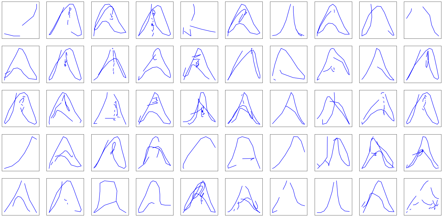
Time for some fun. Let’s use our final model to produce more drawings!
Remember the images are clickable, incase you want to see more.
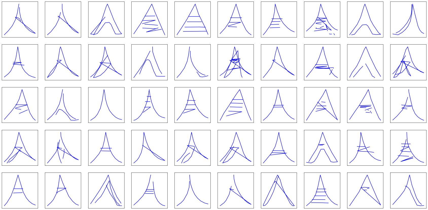
Alright! Eiffel towers and faces won’t get any better.
Now, what about the long-awaited fire trucks?
They look nice enough, but we can do better. Let’s tweak the size of the hidden state, which conditions the complexity of the RNN. Going from $H = 128$ to $H = 512$, with even more drawings (between 30k and 40k drawing instead of 11k), the training lasts around a hour and a half per class of drawings, but results in better fire trucks:
Scale, flashing light, axles. They have it all.
That’s enough metal for now. Let’s turn to more organic stuff.
It is quite obvious what these drawings are.
Now, what better way to close this article than by generating some animals?

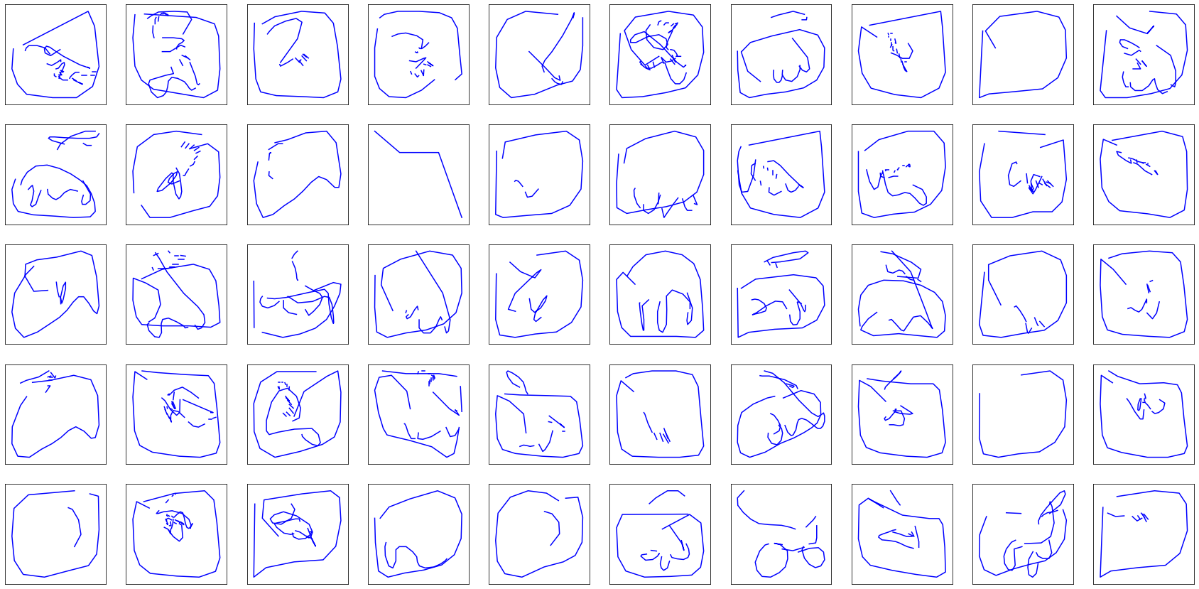
In case you are unsure what the last class of drawings is (either lamas, diplodocuses or random mammals), they are giraffes. While it can quite complicated to recognize them, it is not as bad at it looks, considering the original drawings …
No comment.
Conclusion
In this article, we explored drawings generation using a recurrent neural network by jointly predicting the trajectory, when to lift pencil, and when to stop drawing. Since a vanilla LSTM quickly showed its limit in such an endeavour, we had to stack a probabilistic layer on top of it, making it a mixture density network, that we effectively trained by maximizing the likelihood of the next point under probability distributions shaped by the outputs of the LSTM.
That was quite a journey, but with great results.
From shaky hand-drawn circle, triangle and square primitives in the dataset, the final model generates smooth ones. In the process, it manages to internalize a grammar of drawings, positioning the primitives in such a way that they form recognizable drawings that actually surpass quite a lot of the examples it has been trained on.